
机器学习初使用
1 回归
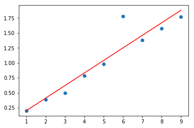
1.1 线性回归 - 最小二乘法拟合
import numpy as np
import matplotlib.pyplot as plt
from IPython.display import Latex,display

print("-"*100)
x = np.array([1,2,3,4,5,6,7,8,9])
y = np.array([0.199,0.389,0.5,0.783,0.980,1.777,1.38,1.575,1.771])

X = np.vstack([x, np.ones(len(x))]).T

print(f'''
X.shape={X.shape}
X={X}
''')
print(f'''
y.shape={y.shape}
y={y}
''')

print("-"*100)
P = np.linalg.lstsq(X, y, rcond=None)[0]   # 最小二乘法
print(f'P.shape={P.shape}')

plt.plot(x, y, 'o', label='original data')
plt.plot(x, P[0] * x + P[1], 'r', label='fitted line')

plt.show()
----------------------------------------------------------------------------------------------------

X.shape=(9, 2)
X=[[1. 1.]
 [2. 1.]
 [3. 1.]
 [4. 1.]
 [5. 1.]
 [6. 1.]
 [7. 1.]
 [8. 1.]
 [9. 1.]]


y.shape=(9,)
y=[0.199 0.389 0.5   0.783 0.98  1.777 1.38  1.575 1.771]

----------------------------------------------------------------------------------------------------
P.shape=(2,)
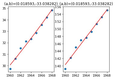
1.2 非线性拟合 - 指数转log,变线性
左图使用线性最小二乘法,右图使用非线性最小二乘法
import numpy as np
import matplotlib.pyplot as plt
from IPython.display import Latex,display
from scipy.optimize import curve_fit


print("-"*100)
t = np.array([1960,1961,1962,1963,1964,1965,1966,1967,1968])
s = np.array([29.72,30.61,31.51,32.13,32.34,32.85,33.56,34.20,34.83])

x = np.array(t)
y = np.log(np.array(s))  # ln
X = np.vstack([x, np.ones(len(x))]).T

print(f'''
X.shape={X.shape}
X={X}
''')
print(f'''
y.shape={y.shape}
y={y}
''')

print("-"*100)
P = np.linalg.lstsq(X, y, rcond=None)[0]   # 线性最小二乘法

plt.subplot(1,2,1)
plt.title('(a,b)=(%f,%f)'%(P[0],P[1]))
plt.plot(t, s, 'o', label='original data')
plt.plot(t, np.exp(P[1])*np.exp(P[0]*t), 'r', label='fitted line')

def func(x,c0,c1):
    return c0+c1*x
popt, pcov = curve_fit(func, x, y)

plt.subplot(1,2,2)
plt.title('(a,b)=(%f,%f)'%(popt[1],popt[0]))
plt.plot(x, y, 'o', label='original data')
plt.plot(x, func(x,*popt), 'r', label='fitted line')

plt.show()
----------------------------------------------------------------------------------------------------

X.shape=(9, 2)
X=[[1.960e+03 1.000e+00]
 [1.961e+03 1.000e+00]
 [1.962e+03 1.000e+00]
 [1.963e+03 1.000e+00]
 [1.964e+03 1.000e+00]
 [1.965e+03 1.000e+00]
 [1.966e+03 1.000e+00]
 [1.967e+03 1.000e+00]
 [1.968e+03 1.000e+00]]


y.shape=(9,)
y=[3.39182022 3.42132675 3.45030496 3.46979017 3.47630485 3.49195174
 3.51333488 3.53222564 3.55047908]

----------------------------------------------------------------------------------------------------
2 聚类
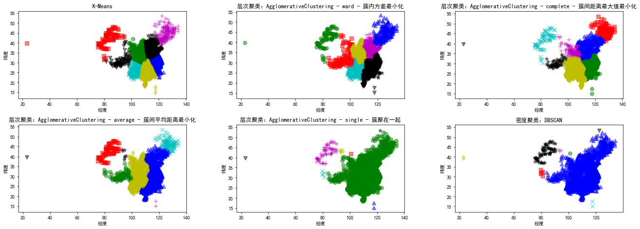
2.1 各种聚类算法
K-Means算法 层次聚类算法:AgglomerativeClustering 密度聚类算法:DBSCAN
import numpy as np
import matplotlib.pyplot as plt
from IPython.display import Latex,display
from sklearn.cluster import KMeans,AgglomerativeClustering,DBSCAN

# 显示中文
def conf_zh(font_name):
    from pylab import mpl
    mpl.rcParams['font.sans-serif'] = [font_name]
    mpl.rcParams['axes.unicode_minus'] = False

conf_zh('SimHei')

x = []
f = open('city.txt',encoding='utf-8')
for v in f:
    #print(v)
    if not v.startswith('城'):
        continue
    else:
        x.append([float(v.split(':')[2].split(' ')[0]), float(v.split(':')[3].split(';')[0])])

x_y = np.array(x)
print(f'''
x_y={x_y}
''')

n_clusters = 8  # 分类数,也就是K值
markers = [['^','b'],['x','c'],['o','g'],['*','k'],['+','m'],['s','r'],['d','y'],['v','k']]

pltsub = [5,3]
f_index = 1
plt.subplot(pltsub[0],pltsub[1],f_index)
f_index += 1
plt.subplots_adjust(top=4,right=3,hspace=0.3,wspace=0.3)
plt.title('K-Means')
cls = KMeans(n_clusters).fit(x_y)

# test 布尔数组
members = cls.labels_ == 3
print(f'members={members}')

for i in range(n_clusters):
    members = cls.labels_ == i
    # 利用布尔索引,只抓取True的出来展示
    plt.scatter(x_y[members,0],x_y[members,1],s=60,marker=markers[i][0], c=markers[i][1], alpha=0.5)
plt.xlabel('经度')
plt.ylabel('纬度')

plt.subplot(pltsub[0],pltsub[1],f_index)
f_index += 1
plt.title('层次聚类:AgglomerativeClustering - ward - 簇内方差最小化')
cls = AgglomerativeClustering(linkage='ward',n_clusters=n_clusters).fit(x)
for i in range(n_clusters):
    members = cls.labels_ == i
    # 利用布尔索引,只抓取True的出来展示
    plt.scatter(x_y[members,0],x_y[members,1],s=60,marker=markers[i][0], c=markers[i][1], alpha=0.5)

plt.xlabel('经度')
plt.ylabel('纬度')

plt.subplot(pltsub[0],pltsub[1],f_index)
f_index += 1
plt.title('层次聚类:AgglomerativeClustering - complete - 簇间距离最大值最小化')
cls = AgglomerativeClustering(linkage='complete',n_clusters=n_clusters).fit(x)
for i in range(n_clusters):
    members = cls.labels_ == i
    # 利用布尔索引,只抓取True的出来展示
    plt.scatter(x_y[members,0],x_y[members,1],s=60,marker=markers[i][0], c=markers[i][1], alpha=0.5)
plt.xlabel('经度')
plt.ylabel('纬度')

plt.subplot(pltsub[0],pltsub[1],f_index)
f_index += 1
plt.title('层次聚类:AgglomerativeClustering - average - 簇间平均距离最小化')
cls = AgglomerativeClustering(linkage='average',n_clusters=n_clusters).fit(x)
for i in range(n_clusters):
    members = cls.labels_ == i
    # 利用布尔索引,只抓取True的出来展示
    plt.scatter(x_y[members,0],x_y[members,1],s=60,marker=markers[i][0], c=markers[i][1], alpha=0.5)
plt.xlabel('经度')
plt.ylabel('纬度')

plt.subplot(pltsub[0],pltsub[1],f_index)
f_index += 1
plt.title('层次聚类:AgglomerativeClustering - single - 簇聚在一起')
cls = AgglomerativeClustering(linkage='single',n_clusters=n_clusters).fit(x)
for i in range(n_clusters):
    members = cls.labels_ == i
    # 利用布尔索引,只抓取True的出来展示
    plt.scatter(x_y[members,0],x_y[members,1],s=60,marker=markers[i][0], c=markers[i][1], alpha=0.5)

plt.xlabel('经度')
plt.ylabel('纬度')

plt.subplot(pltsub[0],pltsub[1],f_index)
f_index += 1
plt.title('密度聚类:DBSCAN')
cls = DBSCAN(eps=2.5,min_samples=1).fit(x)
n_clusters_dbscan = len(set(cls.labels_))
print(f'clusters={n_clusters_dbscan}')
for i in range(n_clusters_dbscan):
    members = cls.labels_ == i
    # 利用布尔索引,只抓取True的出来展示
    plt.scatter(x_y[members,0],x_y[members,1],s=60,marker=markers[i][0], c=markers[i][1], alpha=0.5)

plt.xlabel('经度')
plt.ylabel('纬度')

plt.show()
x_y=[[121.48  31.22]
 [121.24  31.4 ]
 [121.48  31.41]
 ...
 [126.6   51.72]
 [124.7   52.32]
 [122.37  53.48]]

members=[False False False ... False False False]
clusters=8
2.2 聚类评估 - 聚类趋势评估
指标:对于给定数据集,是否有聚类趋势,0.5附近通常不具有聚类趋势,1附近通常存在聚类趋势 方法:霍普金斯统计量—-评估空间中点的密度疏散程度,如果空间中点过于均衡,则最后分类的准确性的误差通常会比较大,因为不具有聚类效应
import numpy as np
import matplotlib.pyplot as plt
from IPython.display import Latex,display
from sklearn.cluster import KMeans,AgglomerativeClustering,DBSCAN

# 显示中文
def conf_zh(font_name):
    from pylab import mpl
    mpl.rcParams['font.sans-serif'] = [font_name]
    mpl.rcParams['axes.unicode_minus'] = False

conf_zh('SimHei')

print('霍普金斯统计量:')

x = []
f = open('city.txt',encoding='utf-8')
for v in f:
    #print(v)
    if not v.startswith('城'):
        continue
    else:
        x.append([float(v.split(':')[2].split(' ')[0]), float(v.split(':')[3].split(';')[0])])

x_y = np.array(x)

# 随机选取3个向量
pn = x_y[np.random.choice(x_y.shape[0],3,replace=False),:]
print(f'''
pn={pn}
''')

xn = []
for i in pn:
    distance_min = 1000000
    for j in x_y:
        if np.array_equal(j, i):
            continue
        distance = np.linalg.norm(j - i)
        if distance_min > distance:
            distance_min = distance
    xn.append(distance_min)

print(f'''
xn={xn}
''')

#接着随机选3个向量
qn = x_y[np.random.choice(x_y.shape[0],3,replace=False),:]
print(f'''
pn={pn}
''')

yn = []
for i in pn:
    distance_min = 1000000
    for j in x_y:
        if np.array_equal(j, i):
            continue
        distance = np.linalg.norm(j - i)
        if distance_min > distance:
            distance_min = distance
    yn.append(distance_min)

print(f'''
yn={yn}
''')

H = float(np.sum(yn)) / (np.sum(xn) + np.sum(yn))
print(f'''
H={H}
''')
霍普金斯统计量:


pn=[[124.7   42.77]
 [119.06  27.61]
 [105.92  26.25]]


xn=[0.49244289008980613, 0.30083217912983207, 0.18384776310850404]


pn=[[124.7   42.77]
 [119.06  27.61]
 [105.92  26.25]]


yn=[0.49244289008980613, 0.30083217912983207, 0.18384776310850404]


H=0.5
2.3 聚类评估 - 类簇数确定
指标:类簇内距离个类簇中心向量的距离和之和达到拐点 方法:肘方法
import numpy as np
import matplotlib.pyplot as plt
from IPython.display import Latex,display
from sklearn.cluster import KMeans,AgglomerativeClustering,DBSCAN
from matplotlib.ticker import MultipleLocator
# 显示中文
def conf_zh(font_name):
from pylab import mpl
mpl.rcParams['font.sans-serif'] = [font_name]
mpl.rcParams['axes.unicode_minus'] = False
conf_zh('SimHei')
x = []
f = open('city.txt',encoding='utf-8')
for v in f:
#print(v)
if not v.startswith('城'):
continue
else:
x.append([float(v.split(':')[2].split(' ')[0]), float(v.split(':')[3].split(';')[0])])
x_y = np.array(x)
print(f'''
x_y={x_y}
''')
def manhattan_distance(x,y):
return np.sum(abs(x-y))
def cluster_distance_sum(n_clusters):
cls = KMeans(n_clusters).fit(x_y)
#print(f'cluster_centers={cls.cluster_centers_}')
distance_sum = 0
for i in range(n_clusters):
group = cls.labels_ ==i
members = x_y[group,:]
for v in members:
distance_sum += manhattan_distance(np.array(v),cls.cluster_centers_[i])
#print(f'distance_sum={distance_sum}')
return distance_sum
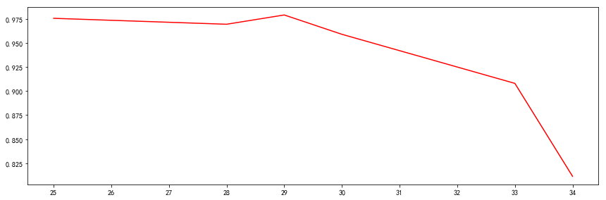
d = []
m = np.arange(1,21,1)
for i in m:
#print(f'clusters={i}')
d.append(cluster_distance_sum(i))
d = np.array(d)
# 显示设置
xmajorLocator = MultipleLocator(1)
ax = plt.subplot(1,1,1)
plt.subplots_adjust(top=1,right=2)
ax.xaxis.set_major_locator(xmajorLocator)
plt.plot(m, d, 'r')
plt.show()
x_y=[[121.48  31.22]
 [121.24  31.4 ]
 [121.48  31.41]
 ...
 [126.6   51.72]
 [124.7   52.32]
 [122.37  53.48]]
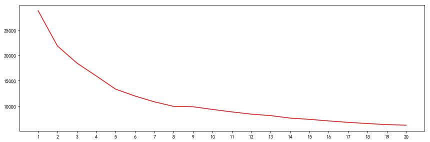
由上述曲线,可知,K取2、5、8、12时,是拐点
2.4 聚类评估 - 聚类质量评估
目标:聚类准确与否 方法:轮廓系数—外在方法是使用已知准确分类来评估质量,但是聚类是无监督的学习,无基准的情况,使用内在方法
import numpy as np
import matplotlib.pyplot as plt
from IPython.display import Latex,display
from sklearn.cluster import KMeans,AgglomerativeClustering,DBSCAN
from matplotlib.ticker import MultipleLocator

# 显示中文
def conf_zh(font_name):
    from pylab import mpl
    mpl.rcParams['font.sans-serif'] = [font_name]
    mpl.rcParams['axes.unicode_minus'] = False

conf_zh('SimHei')

print('轮廓系数:')

x = []
f = open('city.txt',encoding='utf-8')
for v in f:
    #print(v)
    if not v.startswith('城'):
        continue
    else:
        x.append([float(v.split(':')[2].split(' ')[0]), float(v.split(':')[3].split(';')[0])])

x_y = np.array(x)
print(f'''
x_y={x_y}
''')

def manhattan_distance(x,y):
    return np.sum(abs(x-y))

def cacl_kmeans_lunkuo(n_clusters):
    cls = KMeans(n_clusters).fit(x_y)

    # 选x_y[0]作为这个v向量
    # 先计算a(v)
    # 首先知道x_y[0]是属于cls.labels_[0]这个分类的
    group_0 = cls.labels_ == cls.labels_[0]
    group_0_members = x_y[group_0,:]
    distance_sum = 0
    for v in group_0_members[1:]:
        distance_sum += manhattan_distance(x_y[0],np.array(v))
    av = distance_sum / len(group_0_members[1:])

    # 然后计算b(v)
    distance_sum = 0
    distance_min = 100000
    for i in range(n_clusters):
        if i == cls.labels_[0]:
            continue
        group = cls.labels_ == i
        members = x_y[group,:]
        for v in members:
            distance = manhattan_distance(np.array(x_y[0]),np.array(v))
            if distance < distance_min:
                distance_min = distance
        distance_sum += distance_min
    bv = distance_sum / (n_clusters-1)
    sv = float(bv-av) / max(bv,av)
    return av,bv,sv

#n_clusters = 2
m = np.arange(2,21,1)
s = []
for i in m:
    n_clusters = i
    #print(f'clusters={n_clusters}')
    av,bv,sv = cacl_kmeans_lunkuo(n_clusters)
    #print(f'''
    #av={av}
    #bv={bv}
    #sv={sv}
    #''')
    s.append(sv)

xmajorLocator = MultipleLocator(1)
ax = plt.subplot(1,1,1)
plt.subplots_adjust(top=1,right=2)
ax.xaxis.set_major_locator(xmajorLocator)
plt.plot(m,s,'r')
plt.show()
轮廓系数:


x_y=[[121.48  31.22]
 [121.24  31.4 ]
 [121.48  31.41]
 ...
 [126.6   51.72]
 [124.7   52.32]
 [122.37  53.48]]
3 分类
3.1 朴素贝叶斯分类
3.1.1 天气预测
import numpy as np
import matplotlib.pyplot as plt
from IPython.display import Latex,display
from sklearn.naive_bayes import GaussianNB

# 显示中文
def conf_zh(font_name):
    from pylab import mpl
    mpl.rcParams['font.sans-serif'] = [font_name]
    mpl.rcParams['axes.unicode_minus'] = False

conf_zh('SimHei')

# 0:晴  1:阴  2:降水  3:多云
data_table = [['date','weather'],
              [1,0],
              [2,1],
              [3,2],
              [4,1],
              [5,2],
              [6,0],
              [7,0],
              [8,3],
              [9,1],
              [10,1]]

# 当天的天气,最后一天不要算进来,用来作为第二天的数据
X = []
for e in data_table[1:-1]:
    X.append(e[1])
X = np.array(X).reshape(9,1)
print(f'X={X}')

# 当天的天气对应的后一天的天气
y = []
for e in data_table[2:]:
    y.append(e[1])
print(f'y={y}')

clf = GaussianNB().fit(X, y)

p = [[1]]
np.set_printoptions(suppress=True)  # 去掉科学计数法显示
print(f'''
预测概率矩阵=
{np.array(clf.predict_proba(X))}
''')
print(f'''
预测当天阴天,第二天天气[0:晴  1:阴  2:降水  3:多云]
{clf.predict(p)}
''')
print(f'''
预测当天阴天,第二天天气概率矩阵:[0:晴  1:阴  2:降水  3:多云]
{clf.predict_proba(p)}
''')
p=[[3]]
print(f'''
预测当天多云,第二天天气[0:晴  1:阴  2:降水  3:多云]
{clf.predict(p)}
''')
print(f'''
预测当天多云,第二天天气概率矩阵:[0:晴  1:阴  2:降水  3:多云]
{clf.predict_proba(p)}
''')
p=[[0]]
print(f'''
预测当天晴,第二天天气[0:晴  1:阴  2:降水  3:多云]
{clf.predict(p)}
''')
print(f'''
预测当天晴,第二天天气概率矩阵:[0:晴  1:阴  2:降水  3:多云]
{clf.predict_proba(p)}
''')
X=[[0]
 [1]
 [2]
 [1]
 [2]
 [0]
 [0]
 [3]
 [1]]
y=[1, 2, 1, 2, 0, 0, 3, 1, 1]

预测概率矩阵=
[[0.00003812 0.00004571 0.         0.99991617]
 [0.00003142 0.00005086 0.99991771 0.        ]
 [0.2725793  0.7274207  0.         0.        ]
 [0.00003142 0.00005086 0.99991771 0.        ]
 [0.2725793  0.7274207  0.         0.        ]
 [0.00003812 0.00004571 0.         0.99991617]
 [0.00003812 0.00004571 0.         0.99991617]
 [0.15688697 0.84311303 0.         0.        ]
 [0.00003142 0.00005086 0.99991771 0.        ]]


预测当天阴天,第二天天气[0:晴  1:阴  2:降水  3:多云]
[2]


预测当天阴天,第二天天气概率矩阵:[0:晴  1:阴  2:降水  3:多云]
[[0.00003142 0.00005086 0.99991771 0.        ]]


预测当天多云,第二天天气[0:晴  1:阴  2:降水  3:多云]
[1]


预测当天多云,第二天天气概率矩阵:[0:晴  1:阴  2:降水  3:多云]
[[0.15688697 0.84311303 0.         0.        ]]


预测当天晴,第二天天气[0:晴  1:阴  2:降水  3:多云]
[3]


预测当天晴,第二天天气概率矩阵:[0:晴  1:阴  2:降水  3:多云]
[[0.00003812 0.00004571 0.         0.99991617]]
3.1.1 疾病预测
import numpy as np
import matplotlib.pyplot as plt
from IPython.display import Latex,display
from sklearn.naive_bayes import GaussianNB

# 显示中文
def conf_zh(font_name):
    from pylab import mpl
    mpl.rcParams['font.sans-serif'] = [font_name]
    mpl.rcParams['axes.unicode_minus'] = False

conf_zh('SimHei')

np.set_printoptions(suppress=True)  # 去掉科学计数法显示

# 1:是  0:否
data_table = [
    ['基因片段A','基因片段B','高血压','胆结石'],
    [1,1,1,0],
    [0,0,0,1],
    [0,1,0,0],
    [1,0,0,0],
    [1,1,0,1],
    [1,0,0,1],
    [0,1,1,1],
    [0,0,0,0],
    [1,0,1,0],
    [0,1,0,1]
]

X = []   # 基因片段
y1 = []  # 高血压
y2 = []  # 胆结石
for e in data_table[1:]:
    X.append(e[0:2])
    y1.append(e[2:3])
    y2.append(e[3:])

X = np.array(X).reshape(len(X),2)
y1 = np.array(y1).reshape(len(y1),)
y2 = np.array(y2).reshape(len(y2),)

print(f'''
X = {X}
y1 = {y1}
y2 = {y2}
''')

clf_y1 = GaussianNB().fit(X,y1)
clf_y2 = GaussianNB().fit(X,y2)

p = [[1,0]]
print(f'''
高血压预测概率矩阵=
{np.array(clf_y1.predict_proba(X))}

胆结石预测概率矩阵=
{np.array(clf_y2.predict_proba(X))}
''')
print(f'''
预测基因片段AB为{p}:
会得高血压么[1:是  0:否]
{clf_y1.predict(p)}
会得胆结石么[1:是  0:否]
{clf_y2.predict(p)}
''')
print(f'''
预测基因片段AB为{p}:
会得高血压概率矩阵:[1:是  0:否]
{clf_y1.predict_proba(p)}
会得胆结石概率矩阵:[1:是  0:否]
{clf_y2.predict_proba(p)}
''')

p = [[0,1]]
print(f'''
高血压预测概率矩阵=
{np.array(clf_y1.predict_proba(X))}

胆结石预测概率矩阵=
{np.array(clf_y2.predict_proba(X))}
''')
print(f'''
预测基因片段AB为{p}:
会得高血压么[1:是  0:否]
{clf_y1.predict(p)}
会得胆结石么[1:是  0:否]
{clf_y2.predict(p)}
''')
print(f'''
预测基因片段AB为{p}:
会得高血压概率矩阵:[1:是  0:否]
{clf_y1.predict_proba(p)}
会得胆结石概率矩阵:[1:是  0:否]
{clf_y2.predict_proba(p)}
''')

p = [[1,1]]
print(f'''
高血压预测概率矩阵=
{np.array(clf_y1.predict_proba(X))}

胆结石预测概率矩阵=
{np.array(clf_y2.predict_proba(X))}
''')
print(f'''
预测基因片段AB为{p}:
会得高血压么[1:是  0:否]
{clf_y1.predict(p)}
会得胆结石么[1:是  0:否]
{clf_y2.predict(p)}
''')
print(f'''
预测基因片段AB为{p}:
会得高血压概率矩阵:[1:是  0:否]
{clf_y1.predict_proba(p)}
会得胆结石概率矩阵:[1:是  0:否]
{clf_y2.predict_proba(p)}
''')
X = [[1 1]
 [0 0]
 [0 1]
 [1 0]
 [1 1]
 [1 0]
 [0 1]
 [0 0]
 [1 0]
 [0 1]]
y1 = [1 0 0 0 0 0 1 0 1 0]
y2 = [0 1 0 0 1 1 1 0 0 1]


高血压预测概率矩阵=
[[0.47921218 0.52078782]
 [0.88081116 0.11918884]
 [0.72281486 0.27718514]
 [0.72281486 0.27718514]
 [0.47921218 0.52078782]
 [0.72281486 0.27718514]
 [0.72281486 0.27718514]
 [0.88081116 0.11918884]
 [0.72281486 0.27718514]
 [0.72281486 0.27718514]]

胆结石预测概率矩阵=
[[0.5        0.5       ]
 [0.5        0.5       ]
 [0.30294072 0.69705928]
 [0.69705928 0.30294072]
 [0.5        0.5       ]
 [0.69705928 0.30294072]
 [0.30294072 0.69705928]
 [0.5        0.5       ]
 [0.69705928 0.30294072]
 [0.30294072 0.69705928]]


预测基因片段AB为[[1, 0]]:
会得高血压么[1:是  0:否]
[0]
会得胆结石么[1:是  0:否]
[0]


预测基因片段AB为[[1, 0]]:
会得高血压概率矩阵:[1:是  0:否]
[[0.72281486 0.27718514]]
会得胆结石概率矩阵:[1:是  0:否]
[[0.69705928 0.30294072]]


高血压预测概率矩阵=
[[0.47921218 0.52078782]
 [0.88081116 0.11918884]
 [0.72281486 0.27718514]
 [0.72281486 0.27718514]
 [0.47921218 0.52078782]
 [0.72281486 0.27718514]
 [0.72281486 0.27718514]
 [0.88081116 0.11918884]
 [0.72281486 0.27718514]
 [0.72281486 0.27718514]]

胆结石预测概率矩阵=
[[0.5        0.5       ]
 [0.5        0.5       ]
 [0.30294072 0.69705928]
 [0.69705928 0.30294072]
 [0.5        0.5       ]
 [0.69705928 0.30294072]
 [0.30294072 0.69705928]
 [0.5        0.5       ]
 [0.69705928 0.30294072]
 [0.30294072 0.69705928]]


预测基因片段AB为[[0, 1]]:
会得高血压么[1:是  0:否]
[0]
会得胆结石么[1:是  0:否]
[1]


预测基因片段AB为[[0, 1]]:
会得高血压概率矩阵:[1:是  0:否]
[[0.72281486 0.27718514]]
会得胆结石概率矩阵:[1:是  0:否]
[[0.30294072 0.69705928]]


高血压预测概率矩阵=
[[0.47921218 0.52078782]
 [0.88081116 0.11918884]
 [0.72281486 0.27718514]
 [0.72281486 0.27718514]
 [0.47921218 0.52078782]
 [0.72281486 0.27718514]
 [0.72281486 0.27718514]
 [0.88081116 0.11918884]
 [0.72281486 0.27718514]
 [0.72281486 0.27718514]]

胆结石预测概率矩阵=
[[0.5        0.5       ]
 [0.5        0.5       ]
 [0.30294072 0.69705928]
 [0.69705928 0.30294072]
 [0.5        0.5       ]
 [0.69705928 0.30294072]
 [0.30294072 0.69705928]
 [0.5        0.5       ]
 [0.69705928 0.30294072]
 [0.30294072 0.69705928]]


预测基因片段AB为[[1, 1]]:
会得高血压么[1:是  0:否]
[1]
会得胆结石么[1:是  0:否]
[0]


预测基因片段AB为[[1, 1]]:
会得高血压概率矩阵:[1:是  0:否]
[[0.47921218 0.52078782]]
会得胆结石概率矩阵:[1:是  0:否]
[[0.5 0.5]]
3.2 决策树归纳
依据原理是:选择某一个字段作为根,能使得切分次数变少(树的层次变少),则为最佳。此过程递归进行 数据原理:字段划分规则下,用某个字段作为树根,信息熵越大,说明信息越混乱,需要切分次数就越多(第一次没有把关键的二分,则会进行很多次,层次会变多) 目标:用某个字段作为树根,需要选取信息熵最小的那个作为最优值。要使信息熵最小,就要使得信息增益最大化(信息增益:即互信息,表示信号经过系统信息丢失的量,增益越大,说明信息丢失的越多,结果也就越明确)
import numpy as np
import matplotlib.pyplot as plt
from IPython.display import Latex,display
from sklearn.naive_bayes import GaussianNB
from matplotlib.ticker import MultipleLocator
# 显示中文
def conf_zh(font_name):
from pylab import mpl
mpl.rcParams['font.sans-serif'] = [font_name]
mpl.rcParams['axes.unicode_minus'] = False
conf_zh('SimHei')
np.set_printoptions(suppress=True) # 去掉科学计数法显示
# 学历分类中,大专、本科、硕士占比
education = (2.0/12, 5.0/12, 5.0/12)
# 大专分类中,相亲占比
junior_college = (1.0/2, 1.0/2)
# 本科分类中,相亲占比
undergraduate = (3.0/5, 2.0/5)
#硕士分类中,相亲占比
master = (4.0/5, 1.0/5)
# 学历各分类中,相亲占比
date_per = (junior_college, undergraduate, master)
# 相亲字段划分规则下的熵
def info_date(p):
info = 0
for v in p:
info += v * np.log2(v)
return info
# 使用学历字段划分规则下的熵
def infoEdu():
info = 0
for i in range(len(education)):
info += -education[i] * info_date(date_per[i])
return info
print(f'''
学历字段划分的信息熵:
{infoEdu()}
''')
# 年龄
age = np.array([25,25,28,28,29,30,33,34,35,36,40,46])
# 是否相亲 1:是 0:否
date = np.array([0,1,1,0,1,1,1,1,1,0,0,0])
def cacl_infoAge(age_cut):
group_left = age<=age_cut
group_right = age>age_cut
split_per = (float(len(age[group_left]))/len(age), float(len(age[group_right]))/len(age))
# print(split_per)
# 左边分类中相亲占比
group_date = date[group_left] == 1
group_not_date = date[group_left] == 0
date_left = (float(len(date[:len(date[group_left])][group_date]))/len(date[group_left]), float(len(date[:len(date[group_left])][group_not_date]))/len(date[group_left]))
# 右边分类中相亲占比
group_date = date[group_right] == 1
group_not_date = date[group_right] == 0
date_right = (float(len(date[len(date[group_left]):][group_date]))/len(date[group_right]), float(len(date[len(date[group_left]):][group_not_date]))/len(date[group_right]))
#print(date_left)
#print(date_right)
# 左右各分类相亲占比
date_per = (date_left, date_right)
# 左右各分类划分规则下的熵
def infoAge():
info = 0
for i in range(len(split_per)):
info += -split_per[i] * info_date(date_per[i])
return info
return infoAge()
infoAgeValue = []
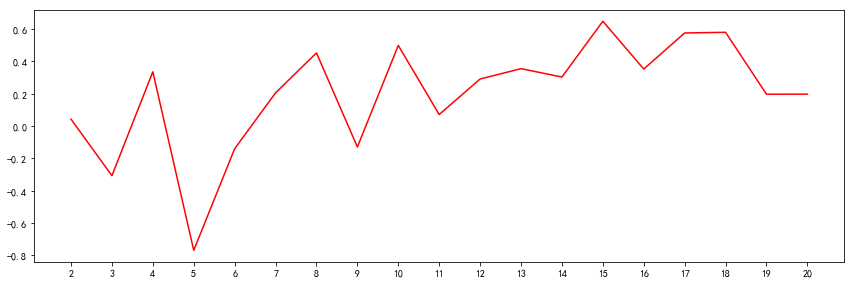
print('年龄字段划分的信息熵')
for i in age[1:-4]:
info = cacl_infoAge(i)
print(info)
infoAgeValue.append(info)
xmajorLocator = MultipleLocator(1)
ax = plt.subplot(1,1,1)
plt.subplots_adjust(top=1,right=2)
ax.xaxis.set_major_locator(xmajorLocator)
plt.plot(age[1:-4], infoAgeValue, 'r')
plt.show()
学历字段划分的信息熵:
0.8720327872258462

年龄字段划分的信息熵
0.9757921620455572
0.9696226686166431
0.9696226686166431
0.979279160376092
0.9591479170272448
0.9080497460199801
0.8112781244591328
由于在34岁以后,无相亲的,所以这些是垃圾数据,可以排除掉。而在34岁年龄熵达到最小值,比学历要重,因此选年龄且按照34划分是目前看起来最合适作为根的
3.3 随机森林
import numpy as np
import matplotlib.pyplot as plt
from IPython.display import Latex,display
from sklearn.naive_bayes import GaussianNB
from matplotlib.ticker import MultipleLocator
from sklearn.ensemble import RandomForestClassifier

# 显示中文
def conf_zh(font_name):
    from pylab import mpl
    mpl.rcParams['font.sans-serif'] = [font_name]
    mpl.rcParams['axes.unicode_minus'] = False

conf_zh('SimHei')

np.set_printoptions(suppress=True)  # 去掉科学计数法显示

# 学历: 0:大专  1:本科  2:硕士
# 年龄、身高、年收入、学历
x = [
    [25,179,15,0],
    [33,190,19,0],
    [28,180,18,2],
    [25,178,18,2],
    [46,100,100,2],
    [40,170,170,1],
    [34,174,20,2],
    [35,181,55,1],
    [35,170,25,2],
    [30,180,35,1],
    [28,174,30,1],
    [29,176,36,1]
]

# 有否相亲 0:N  1:Y
y = [0,1,1,1,0,0,1,0,1,1,0,1]

print(f'''
x = {x}
y = {y}
''')

clf = RandomForestClassifier(n_estimators=100).fit(x,y)

p = [[28,180,18,2]]
print(f'''
相亲预测概率矩阵=
{np.array(clf.predict_proba(x))}
''')
print(f'''
预测人属性为{p}:
是否相亲[1:是  0:否]
{clf.predict(p)}
''')
x = [[25, 179, 15, 0], [33, 190, 19, 0], [28, 180, 18, 2], [25, 178, 18, 2], [46, 100, 100, 2], [40, 170, 170, 1], [34, 174, 20, 2], [35, 181, 55, 1], [35, 170, 25, 2], [30, 180, 35, 1], [28, 174, 30, 1], [29, 176, 36, 1]]
y = [0, 1, 1, 1, 0, 0, 1, 0, 1, 1, 0, 1]


相亲预测概率矩阵=
[[0.67 0.33]
 [0.15 0.85]
 [0.1  0.9 ]
 [0.09 0.91]
 [0.86 0.14]
 [0.89 0.11]
 [0.06 0.94]
 [0.63 0.37]
 [0.16 0.84]
 [0.1  0.9 ]
 [0.64 0.36]
 [0.24 0.76]]


预测人属性为[[28, 180, 18, 2]]:
是否相亲[1:是  0:否]
[1]
3.4 隐马尔可夫模型
跟上下文有关系的场景,非常适合用到。比如语言识别、自然语言处理等
相关问题: 问题1:知道结果,也知道得到这个结果的各种方法路径及概率,想推测出得到这个结果经过的最佳方法路径 问题2:知道结果,也知道得到这个结果的各种方法路径及概率,想推测出得到这个结果的概率 问题3:知道结果,也知道得到结果经过的路径,想知道每种路径的概率
import numpy as np
import matplotlib.pyplot as plt
from IPython.display import Latex,display
from sklearn.naive_bayes import GaussianNB
from matplotlib.ticker import MultipleLocator
from sklearn.ensemble import RandomForestClassifier

# 显示中文
def conf_zh(font_name):
    from pylab import mpl
    mpl.rcParams['font.sans-serif'] = [font_name]
    mpl.rcParams['axes.unicode_minus'] = False

conf_zh('SimHei')

np.set_printoptions(suppress=True)  # 去掉科学计数法显示

jin = ['近','斤','今','金','尽']
jin_per = [0.3, 0.2, 0.1, 0.06, 0.03]
jintian = ['天','填','田','甜','添']
jintian_per = [
    [0.001, 0.001, 0.001, 0.001, 0.001],
    [0.001, 0.001, 0.001, 0.001, 0.001],
    [0.990, 0.001, 0.001, 0.001, 0.001],
    [0.002, 0.001, 0.850, 0.001, 0.001],
    [0.001, 0.001, 0.001, 0.001, 0.001]
]

wo = ['我','窝','喔','握','卧']
wo_per = [0.400, 0.150, 0.090, 0.050, 0.030]
women = ['们','门','闷','焖','扪']
women_per = [
    [0.970, 0.001, 0.003, 0.001, 0.001],
    [0.001, 0.001, 0.001, 0.001, 0.001],
    [0.001, 0.001, 0.001, 0.001, 0.001],
    [0.001, 0.001, 0.001, 0.001, 0.001],
    [0.001, 0.001, 0.001, 0.001, 0.001]
]

N = 5

def found_from_oneword(oneword_per):
    index = []
    values = []
    a = np.array(oneword_per)
    for v in np.argsort(a)[::-1][:N]:
        index.append(v)
        values.append(oneword_per[v])
    return index, values

def found_from_twoword(oneword_per, twoword_per):
    last = 0
    for i in range(len(oneword_per)):
        current = np.multiply(oneword_per[i], twoword_per[i])
        if i == 0:
            last = current
        else:
            last = np.concatenate((last, current), axis = 0)
    index = []
    values = []
    for v in np.argsort(last)[::-1][:N]:
        index.append([int(v / 5), int(v % 5)])
        values.append(last[v])
    return index, values

def predict(word):
    if word == 'jin':
        for i in found_from_oneword(jin_per)[0]:
            print(jin[i])
    elif word == 'jintian':
        for i in found_from_twoword(jin_per, jintian_per)[0]:
            print(jin[i[0]] + jintian[i[1]])
    elif word == 'wo':
        for i in found_from_oneword(wo_per)[0]:
            print(wo[i])
    elif word == 'women':
        for i in found_from_twoword(wo_per, women_per)[0]:
            print(wo[i[0]] + women[i[1]])
    elif word == 'jintianwo':
        index1, value1 = found_from_oneword(wo_per)
        index2, value2 = found_from_twoword(jin_per, jintian_per)
        last = np.multiply(value1, value2)
        for i in np.argsort(last)[::-1][:N]:
            print(jin[index2[i][0]], jintian[index2[i][1]], wo[i])
    elif word == 'jintianwomen':
        index1, value1 = found_from_twoword(jin_per, jintian_per)
        index2, value2 = found_from_twoword(wo_per, women_per)
        last = np.multiply(value1, value2)
        for i in np.argsort(last)[::-1][:N]:
            print(jin[index1[i][0]], jintian[index1[i][1]], wo[index2[i][0]], women[index2[i][1]])

if __name__ == '__main__':
    predict('jin')
    predict('jintian')
    predict('wo')
    predict('women')
    predict('jintianwo')
    predict('jintianwomen')
近
斤
今
金
尽
今天
金田
近天
近填
近田
我
窝
喔
握
卧
我们
我闷
我门
我焖
我扪
今 天 我
金 田 窝
近 天 喔
近 填 握
近 田 卧
今 天 我 们
金 田 我 闷
近 田 我 扪
近 填 我 焖
近 天 我 门
3.5 SVM支持向量机
通用分类算法 核心:升维,使得一维空间不可分,就把分类平面函数映射到二维空间,二维空间投影到一维空间就是我们需要的分类。所有n维问题,都可以映射到n+1维空间去构造分类函数
import numpy as np
import matplotlib.pyplot as plt
from IPython.display import Latex,display
from sklearn.naive_bayes import GaussianNB
from matplotlib.ticker import MultipleLocator
from sklearn.ensemble import RandomForestClassifier
from sklearn import svm

# 显示中文
def conf_zh(font_name):
    from pylab import mpl
    mpl.rcParams['font.sans-serif'] = [font_name]
    mpl.rcParams['axes.unicode_minus'] = False

conf_zh('SimHei')

np.set_printoptions(suppress=True)  # 去掉科学计数法显示

x = [[34],[33],[32],[31],[30],[30],[25],[23],[22],[18]]
y = [1,0,1,0,1,1,0,1,0,1]

clf = svm.SVC(kernel='rbf',probability=True,gamma='scale').fit(x, y)

p = [[30]]
print(f'''
客户质量预测概率矩阵=
{np.array(clf.predict_proba(x))}
''')
print(f'''
预测客户年龄为{p}:
是否优质[1:是  0:否]
{clf.predict(p)}
''')
客户质量预测概率矩阵=
[[0.57935993 0.42064007]
 [0.52648715 0.47351285]
 [0.5        0.5       ]
 [0.52794556 0.47205444]
 [0.57904877 0.42095123]
 [0.57904877 0.42095123]
 [0.21505131 0.78494869]
 [0.3501047  0.6498953 ]
 [0.3305246  0.6694754 ]
 [0.57904877 0.42095123]]


预测客户年龄为[[30]]:
是否优质[1:是  0:否]
[1]
3.6 遗传算法
核心思想是迭代和重组,淘汰劣质 基本过程: (1)基因编码 (2)设计初始群体 (3)适应度计算 (4)生产下一代 (5)迭代计算
3.6.1 背包问题
import numpy as np
import matplotlib.pyplot as plt
import random
from matplotlib.ticker import MultipleLocator

# 背包问题
# 物品编号和重量、价格
x = {
    1: [10,15],
    2: [15,25],
    3: [20,35],
    4: [25,45],
    5: [30,55],
    6: [35,70]
}

# 终止界限
FINISHED_LIMIT = 5
# 重量界限
WEIGHT_LIMIT = 80
# 染色体长度
CHROMOSOME_SIZE = 6
# 遴选次数
SELECT_NUMBER = 4
max_last = 0
diff_last = 10000

# 收敛条件、判断退出
def is_finished(fitnesses):
    global max_last
    global diff_last
    max_current = 0
    for v in fitnesses:
        if v[1] > max_current:
            max_current = v[1]
    diff = max_current - max_last
    if diff < FINISHED_LIMIT and diff_last < FINISHED_LIMIT:
        return True
    else:
        diff_last = diff
        max_last = max_current
    return False

# 初始染色体样态
def init():
    chromosome_state1 = '100100'
    chromosome_state2 = '101010'
    chromosome_state3 = '010101'
    chromosome_state4 = '101011'
    chromosome_states = [chromosome_state1,
                         chromosome_state2,
                         chromosome_state3,
                         chromosome_state4
                        ]
    return chromosome_states

# 计算适应度
def fitness(chromosome_states):
    fitnesses = []
    for chromosome_state in chromosome_states:
        value_sum = 0
        weight_sum = 0
        for i, v in enumerate(chromosome_state):
            if int(v) == 1:
                weight_sum += x[i + 1][0]
                value_sum += x[i + 1][1]
        fitnesses.append([value_sum, weight_sum])
    return fitnesses

# 筛选
def filter(chromosome_states, fitnesses):
    # 重量大于80的被淘汰
    index = len(fitnesses) - 1
    while index >= 0:
        index -= 1
        if fitnesses[index][1] > WEIGHT_LIMIT:
            chromosome_states.pop(index)
            fitnesses.pop(index)
    # 筛选
    selected_index = [0] * len(chromosome_states)
    for i in range(SELECT_NUMBER):
        j = chromosome_states.index(random.choice(chromosome_states))
        selected_index[j] += 1
    return selected_index

# 生产下一代
def crossover(chromosome_states, selected_index):
    chromosome_states_new = []
    index = len(chromosome_states) - 1
    while index >= 0:
        index -= 1
        chromosome_state = chromosome_states.pop(index)
        for i in range(selected_index[index]):
            chromosome_state_x = random.choice(chromosome_states)
            pos = random.choice(range(1, CHROMOSOME_SIZE - 1))
            chromosome_states_new.append(chromosome_state[:pos] + chromosome_state_x[pos:])
        chromosome_states.insert(index, chromosome_state)
    return chromosome_states_new

def max_price(fitnesses):
    return sorted(np.array(fitnesses)[:,0],reverse=True)[0]

if __name__ == '__main__':
    # 初始群体
    x_price = []
    y_price = []
    chromosome_states = init()
    n = 100
    while n > 0:
        n -= 1
        # 适应度计算
        fitnesses = fitness(chromosome_states)
        if is_finished(fitnesses):
            print(n)
            print(fitnesses)
            # 求出chromosome_states中最大价值者
            x_price.append(100 - n)
            y_price.append(max_price(fitnesses))
            break
        # 筛选
        selected_index = filter(chromosome_states, fitnesses)
        # 求出chromosome_states中最大价值者
        x_price.append(100 - n)
        y_price.append(max_price(fitnesses))
        # 产生下一代
        chromosome_states = crossover(chromosome_states, selected_index)
    #print(chromosome_states)
    xmajorLocator = MultipleLocator(1)
    ax = plt.subplot(1,1,1)
    #plt.subplots_adjust(top=1,right=2)
    ax.xaxis.set_major_locator(xmajorLocator)
    plt.plot(x_price,y_price,'r')
    plt.show()
95
[[130, 70], [120, 65], [140, 75], [140, 75]]
遗传算法最大的问题,就是可能会灭绝,能有一个优质股产生是不容易的。上述的结果,最后也是很随机的能抽到140,75也不是百分百的
3.6.2 极大值问题
import random
import math
import numpy as np

# 染色体长度
CHROMOSOME_SIZE = 15

# 收敛条件、判断退出
def is_finished(last_three):
    s = sorted(last_three)
    if s[0] and s[2] - s[0] < 0.001 * s[0]:
        return True
    return False

# 初始染色体样态
def init():
    chromosome_state1 = ['000000100101001', '101010101010101']
    chromosome_state2 = ['011000100101100', '001100110011001']
    chromosome_state3 = ['001000100100101', '101010101010101']
    chromosome_state4 = ['000110100100100', '110011001100110']
    chromosome_state5 = ['100000100100101', '101010101010101']
    chromosome_state6 = ['101000100100100', '111100001111000']
    chromosome_state7 = ['101010100110100', '101010101010101']
    chromosome_state8 = ['100110101101000', '000011110000111']
    chromosome_states = [chromosome_state1,
                     chromosome_state2,
                     chromosome_state3,
                     chromosome_state4,
                     chromosome_state5,
                     chromosome_state6,
                     chromosome_state7,
                     chromosome_state8]
    return chromosome_states

# 计算适应度
def fitness(chromosome_states):
    fitnesses = []
    for chromosome_state in chromosome_states:
        if chromosome_state[0][0] == '1':
            x = 10 * (-float(int(chromosome_state[0][1:],2)-1)/16384)
        else:
            x = 10 * (float(int(chromosome_state[0],2)+1)/16384)
        if chromosome_state[1][0] == '1':
            y = 10 * (-float(int(chromosome_state[1][1:],2)-1)/16384)
        else:
            y = 10 * (float(int(chromosome_state[1],2)+1)/16384)
        z = y * math.sin(x) + x * math.cos(y)
        fitnesses.append(z)
    return fitnesses

# 筛选
def filter(chromosome_states, fitnesses):
    # top 8 对应的索引值
    chromosome_state_new = []
    top1_fitness_index = 0
    for i in np.argsort(fitnesses)[::-1][:8].tolist():
        chromosome_state_new.append(chromosome_states[i])
        top1_fitness_index = i
    return chromosome_state_new, top1_fitness_index

# 生产下一代
def crossover(chromosome_states):
    chromosome_states_new = []
    while chromosome_states:
        chromosome_state = chromosome_states.pop(0)
        for v in chromosome_states:
            pos = random.choice(range(8, CHROMOSOME_SIZE - 1))
            chromosome_states_new.append([chromosome_state[0][:pos] + v[0][pos:], chromosome_state[1][:pos] + v[1][pos:]])
            chromosome_states_new.append([v[0][:pos] + chromosome_state[1][pos:], v[0][:pos] + chromosome_state[1][pos:]])
    return chromosome_states_new

# 基因突变
def mutation(chromosome_states):
    n = int(5.0 / 100 * len(chromosome_states))
    while n > 0:
        n -= 1
        chromosome_state = random.choice(chromosome_states)
        index = chromosome_states.index(chromosome_state)
        pos = random.choice(range(len(chromosome_state)))
        x = chromosome_state[0][:pos] + str(int(not int(chromosome_state[0][pos]))) +chromosome_state[0][pos+1:]
        y = chromosome_state[1][:pos] + str(int(not int(chromosome_state[1][pos]))) +chromosome_state[1][pos+1:]
        chromosome_states[index] = [x,y]

if __name__ == '__main__':
    # 初始群体
    chromosome_states = init()
    last_three = [0] * 3
    last_num = 0
    n = 100
    while n > 0:
        n -= 1
        # 产生下一代
        chromosome_states = crossover(chromosome_states)
        # 基因突变
        mutation(chromosome_states)
        fitnesses = fitness(chromosome_states)
        chromosome_states, top1_fitness_index = filter(chromosome_states, fitnesses)
        last_three[last_num] = fitnesses[top1_fitness_index]
        if is_finished(last_three):
            break
        if last_num >= 2:
            last_num = 0
        else:
            last_num += 1
    print(chromosome_states)
[['011000101000001', '011000101000001'], ['011000101000001', '011000101000001'], ['011000101000001', '011000101000001'], ['011000101000001', '011000101000001'], ['011000101000001', '011000101000001'], ['011000101000001', '011000101000001'], ['011000101000001', '011000101000001'], ['011000101000001', '011000101000001']]
4 文本挖掘
4.1 文本分类
常规步骤: (1)分词 (2)文本表示(归一化、词频统计) (3)分类标记(分词关联到某个分类,常用算法:Rocchio算法、朴素贝叶斯分类、K-近邻算法、决策树、神经网络、支持向量机等)
4.1.1 Rocchio算法
(1)人工确定文档分类 (2)文档分词,并计算每个分词的词频 (3)本文档所有的分词组成一个向量,包含每个分词的概率(权重) (4)做预测,预测分类标准是看对应文档的分词向量与已学习的文档分类的余弦相似度
# coding = utf-8

import numpy as np
import matplotlib.pyplot as plt
from IPython.display import Latex,display
from sklearn.naive_bayes import GaussianNB
from matplotlib.ticker import MultipleLocator
from sklearn.ensemble import RandomForestClassifier
from sklearn.datasets import fetch_20newsgroups
from sklearn.feature_extraction.text import CountVectorizer
from sklearn.feature_extraction.text import TfidfTransformer
from pprint import pprint
import ssl
import sys,os,os.path
import gc
#os.environ['HTTP_PROXY']="http://web-proxy.oa.com:8080"
#os.environ['HTTPS_PROXY']="http://web-proxy.oa.com:8080"

ssl._create_default_https_context = ssl._create_unverified_context

np.set_printoptions(suppress=True)  # 去掉科学计数法显示

newsgroups_train = fetch_20newsgroups(subset='train')
pprint(list(newsgroups_train.target_names))

# 选4个分类
categories = ['alt.atheism','comp.graphics','sci.med','soc.religion.christian']

# 下载4个主题的文件
twenty_train = fetch_20newsgroups(subset='train',categories=categories)
count_vect = CountVectorizer()
X_train_counts = count_vect.fit_transform(twenty_train.data)
tfidf_transformer = TfidfTransformer()
x_train_tfidf = tfidf_transformer.fit_transform(X_train_counts)

word = count_vect.get_feature_names()
weight = x_train_tfidf.toarray()
for i in range(min(len(weight),10)):
    #print(u"-------这里输出第",i,u"类文本的词语tf-idf权重------")
    for j in range(min(len(word),11110)):
        if j < 11100:
            continue
        #print(word[j],weight[i][j])

del count_vect,X_train_counts,tfidf_transformer,x_train_tfidf,word,weight
gc.collect()
['alt.atheism',
 'comp.graphics',
 'comp.os.ms-windows.misc',
 'comp.sys.ibm.pc.hardware',
 'comp.sys.mac.hardware',
 'comp.windows.x',
 'misc.forsale',
 'rec.autos',
 'rec.motorcycles',
 'rec.sport.baseball',
 'rec.sport.hockey',
 'sci.crypt',
 'sci.electronics',
 'sci.med',
 'sci.space',
 'soc.religion.christian',
 'talk.politics.guns',
 'talk.politics.mideast',
 'talk.politics.misc',
 'talk.religion.misc']


7